本文由 发布,转载请注明出处,如有问题请联系我们! 发布时间: 2021-05-24技术干货 | 基于MindSpore更好的理解Focal Loss
加载中技术性干货知识 | 根据MindSpore更强的了解Focal Loss
【当期强烈推荐专题讲座】物联网技术从业者必看:华为云服务权威专家给你详尽讲解LiteOS各控制模块开发设计以及完成基本原理。
引言:Focal Loss的2个特性算作关键,实际上便是用一个适合的涵数去衡量难归类和容易归类样版对总的损害的奉献。
文中共享自华为云服务小区《技术性干货知识 | 根据MindSpore更强的了解Focal Loss》,全文创作者:chengxiaoli。
今日升级一下恺明高手的Focal Loss,它是 Kaiming 高手精英团队在她们的毕业论文Focal Loss for Dense Object Detection明确提出来的损失函数,运用它改进了图象物件检验的实际效果。ICCV2017RBG和Kaiming高手的大作(https://arxiv.org/pdf/1708.02002.pdf)。
应用情景
近期一直在做面部小表情有关的方位,这一行业的 DataSet 总数并不大,并且通常存有正负极样版不平衡的难题。一般来说,处理正负极样版总数不平衡难题有两个方式:
1. 设计方案取样对策,一般全是对总数少的样版开展重采样
2. 设计方案 Loss,一般全是对不一样类型样版开展权重值取值
文中讲的是第二种对策中的 Focal Loss。
基础理论剖析
毕业论文剖析
我们知道object detection按其步骤而言,一般分成两类。一类是two stage detector(如十分經典的Faster R-CNN,RFCN那样必须region proposal的检验优化算法),第二类则是one stage detector(如SSD、YOLO系列产品那样不用region proposal,立即重归的检验优化算法)。
针对第一类优化算法能够 做到很高的准确度,可是速率比较慢。尽管能够 根据降低proposal的总数或减少键入图象的屏幕分辨率等方法做到加速,可是速率并沒有质的提高。
针对第二类优化算法速率迅速,可是准确度比不上第一类。
因此 总体目标便是:focal loss的立足点是期待one-stage detector能够 做到two-stage detector的准确度,另外不危害原来的速率。
So,Why?and result?
这是怎么回事导致的呢?the Reason is:Class Imbalance(正负极样版不平衡),样版的类型不平衡造成 的。
我们知道在object detection行业,一张图象很有可能转化成不计其数的candidate locations,可是在其中仅有非常少一部分是包括object的,这就产生了类型不平衡。那麼类型不平衡会产生哪些不良影响呢?引入全文讲的2个不良影响:
(1) training is inefficient as most locations are easy negatives that contribute no useful learning signal;
(2) en masse, the easy negatives can overwhelm training and lead to degenerate models.
含意便是负样版总数很大(归属于情况的样版),占总的loss的绝大多数,并且多是非常容易归类的,因而促使实体模型的提升方位并并不是大家所期待的那般。那样,互联网学不上有效的信息内容,没法对object开展精确归类。实际上此前也是有一些优化算法来解决类型不平衡的难题,例如OHEM(online hard example mining),OHEM的关键观念可以用全文的一句话归纳:In OHEM each example is scored by its loss, non-maximum suppression (nms) is then applied, and a minibatch is constructed with the highest-loss examples。OHEM优化算法尽管提升了错归类样版的权重值,可是OHEM优化算法忽视了非常容易归类的样版。
因而对于类型不平衡难题,创作者明确提出一种新的损失函数:Focal Loss,这一损失函数是在规范交叉熵损失基本上改动获得的。这一涵数能够 根据降低易归类样版的权重值,促使实体模型在训炼时更致力于难归类的样版。为了更好地证实Focal Loss的实效性,创作者设计方案了一个dense detector:RetinaNet,而且在训炼时选用Focal Loss训炼。试验证实RetinaNet不但能够 做到one-stage detector的速率,也可以有two-stage detector的准确度。
公式计算表明
详细介绍focal loss,在详细介绍focal loss以前,先讨论一下交叉熵损失,这儿以二分类为例子,原先的归类loss是每个训练样本交叉熵的立即求饶,也就是每个样版的权重值是一样的。公式计算以下: 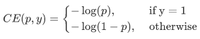 由于是二分类,p表明预测分析样版归属于1的几率(范畴为0-1),y表明label,y的赋值为{ 1,-1}。当真正label是1,也就是y=1时,倘若某一样版x预测分析为1这一类的几率p=0.6,那麼损害便是-log(0.6),留意这一损害是高于或等于0的。假如p=0.9,那麼损害便是-log(0.9),因此 p=0.6的损害要超过p=0.9的损害,这非常容易了解。这儿只是以二分类为例子,多归类归类依此类推为了更好地便捷,用pt替代p,以下公式计算2:。这儿的pt便是前边Figure1中的横坐标轴。
 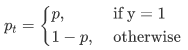 为了更好地表明简单,大家用p_t表明样版归属于true class的几率。因此 (1)式能够 写出:
 ![]() 下面详细介绍一个最基本上的对交叉熵的改善,也将做为文中试验的baseline,即然one-stage detector在训炼的情况下正负极样版的总数差别非常大,那麼一种普遍的作法便是给正负极样版再加上权重值,负样版发生的次数多,那麼就减少负样版的权重值,正样版总数少,就相对性提升正样版的权重值。因而能够 根据设置
下面详细介绍一个最基本上的对交叉熵的改善,也将做为文中试验的baseline,即然one-stage detector在训炼的情况下正负极样版的总数差别非常大,那麼一种普遍的作法便是给正负极样版再加上权重值,负样版发生的次数多,那麼就减少负样版的权重值,正样版总数少,就相对性提升正样版的权重值。因而能够 根据设置 ![]() 的值来操纵正负极样版对总的loss的共享资源权重值。
的值来操纵正负极样版对总的loss的共享资源权重值。 ![]() 取较为小的值来减少负样版(多的那种样版)的权重值。
取较为小的值来减少负样版(多的那种样版)的权重值。 ![]()
显而易见前边的公式计算3尽管能够 操纵正负极样版的权重值,可是无法操纵非常容易归类和难归类样版的权重值,因此就拥有Focal Loss,这儿的γ称之为focusing parameter,γ>=0,称之为调配指数:
![]()
为何要再加上这一调配指数呢?目地是根据降低易归类样版的权重值,进而促使实体模型在训炼时更致力于难归类的样版。
根据试验发觉,绘制图看以下Figure1,横坐标轴是pt,纵轴是loss。CE(pt)表明规范的交叉熵公式计算,FL(pt)表明focal loss中采用的改善的交叉熵。Figure1中γ=0的深蓝色曲线图便是规范的交叉熵损失(loss)。
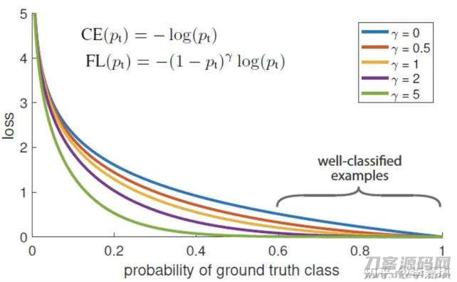
那样就既保证了处理正负极样版不平衡,也保证了处理easy与hard样版不平衡的难题。
结果
创作者将类型不平衡做为阻拦one-stage方式 超出top-performing的two-stage方式 的关键缘故。为了更好地处理这个问题,创作者明确提出了focal loss,在交叉熵里边用一个调节项,为了更好地将学习培训致力于hard examples上边,而且减少很多的easy negatives的权重值。是另外解决了正负极样版不平衡及其区别简易与繁杂样版的难题。
MindSpore编码完成
大家看来一下,根据MindSpore完成Focal Loss的编码:
import mindspore

import mindspore.common.dtype as mstype

from mindspore.common.tensor import Tensor

from mindspore.common.parameter import Parameter

from mindspore.ops import operations as P

from mindspore.ops import functional as F

from mindspore import nn


class FocalLoss(_Loss):


    def __init__(self, weight=None, gamma=2.0, reduction='mean'):

        super(FocalLoss, self).__init__(reduction=reduction)

        # 校检gamma,这儿的γ称之为focusing parameter,γ>=0,称之为调配指数

        self.gamma = validator.check_value_type("gamma", gamma, [float])

        if weight is not None and not isinstance(weight, Tensor):

            raise TypeError("The type of weight should be Tensor, but got {}.".format(type(weight)))

        self.weight = weight

        # 采用的mindspore算法

        self.expand_dims = P.ExpandDims()

        self.gather_d = P.GatherD()

        self.squeeze = P.Squeeze(axis=1)

        self.tile = P.Tile()

        self.cast = P.Cast()


    def construct(self, predict, target):

        targets = target

        # 对键入开展校检

        _check_ndim(predict.ndim, targets.ndim)

        _check_channel_and_shape(targets.shape[1], predict.shape[1])

        _check_predict_channel(predict.shape[1])


        # 将logits和target的样子更改成num_batch * num_class * num_voxels.

        if predict.ndim > 2:

            predict = predict.view(predict.shape[0], predict.shape[1], -1) # N,C,H,W => N,C,H*W

            targets = targets.view(targets.shape[0], targets.shape[1], -1) # N,1,H,W => N,1,H*W or N,C,H*W

        else:

            predict = self.expand_dims(predict, 2) # N,C => N,C,1

            targets = self.expand_dims(targets, 2) # N,1 => N,1,1 or N,C,1


        # 测算多数几率

        log_probability = nn.LogSoftmax(1)(predict)

        # 只保存每一个voxel的路面真值类的多数几率值。

        if target.shape[1] == 1:

            log_probability = self.gather_d(log_probability, 1, self.cast(targets, mindspore.int32))

            log_probability = self.squeeze(log_probability)


        # 获得几率

        probability = F.exp(log_probability)


        if self.weight is not None:

            convert_weight = self.weight[None, :, None]  # C => 1,C,1

            convert_weight = self.tile(convert_weight, (targets.shape[0], 1, targets.shape[2])) # 1,C,1 => N,C,H*W

            if target.shape[1] == 1:

                convert_weight = self.gather_d(convert_weight, 1, self.cast(targets, mindspore.int32))  # selection of the weights  => N,1,H*W

                convert_weight = self.squeeze(convert_weight)  # N,1,H*W => N,H*W

            # 将多数几率乘于他们的权重值

            probability = log_probability * convert_weight

        # 测算损害小批量生产

        weight = F.pows(-probability   1.0, self.gamma)

        if target.shape[1] == 1:

            loss = (-weight * log_probability).mean(axis=1)  # N

        else:

            loss = (-weight * targets * log_probability).mean(axis=-1)  # N,C


        return self.get_loss(loss)
操作方法以下:
from mindspore.common import dtype as mstype

from mindspore import nn

from mindspore import Tensor


predict = Tensor([[0.8, 1.4], [0.5, 0.9], [1.2, 0.9]], mstype.float32)

target = Tensor([[1], [1], [0]], mstype.int32)

focalloss = nn.FocalLoss(weight=Tensor([1, 2]), gamma=2.0, reduction='mean')

output = focalloss(predict, target)

print(output)


0.33365273
Focal Loss的2个关键特性
1. 当一个样版被分错的情况下,pt是不大的,那麼调配因素(1-Pt)贴近1,损害不被危害;当Pt→1,因素(1-Pt)贴近0,那麼分的比较好的(well-classified)样版的权重值就被降低了。因而调配指数就趋向1,换句话说对比原先的loss是没什么大的更改的。当pt趋向1的情况下(这时归类恰当并且是易归类样版),调配指数趋向0,也就是针对总的loss的奉献不大。
2. 当γ=0的情况下,focal loss便是传统式的交叉熵损失,当γ提升的情况下,调配指数也会提升。 潜心主要参数γ光滑地调整了易分样版降低权重值的占比。γ扩大能提高调配因素的危害,试验发觉γ取2最好是。判断力上而言,调配因素降低了易分样版的损害奉献,扩宽了示例接受到低损害的范畴。当γ一定的情况下,例如相当于2,一样easy example(pt=0.9)的loss要比规范的交叉熵loss小100 倍,当pt=0.968时,要小1000 倍,可是针对hard example(pt < 0.5),loss数最多变小4倍。那样的话hard example的权重值相对性就提高了许多。
那样就提升了这些误归类的必要性Focal Loss的2个特性算作关键,实际上便是用一个适合的涵数去衡量难归类和容易归类样版对总的损害的奉献。
加关注,第一时间掌握华为云服务新鮮技术性~